I can (and have) go on and on about the treachery of messy/bad datasets. Though its substantially less exciting than… pretty much everything else, I believe (proportional to the heartache and stress it causes) we don’t spend enough time talking about it or building solutions around it. No matter how new and fancy your ML algorithm is, it’s success is predicated upon a properly sanitized dataset. If you are using bad data, your approach will fail—either flagrantly (best case), or unnoticeably (considerably more probable and considerably more pernicious).

assertr is a R package to help you identify common dataset errors. More specifically, it helps you easily spell out your assumptions about how the data should look and alert you of any deviation from those assumptions.

I’ll return to this point later in the post when we have more background, but I want to be up front about the goals of the package; assertr is not (and can never be) a “one-stop shop” for all of your data validation needs. The specific kind of checks individuals or teams have to perform any particular dataset are often far too idiosyncratic to ever be exhaustively addressed by a single package (although, the assertive meta-package may come very close!) But all of these checks will reuse motifs and follow the same patterns. So, instead, I’m trying to sell assertr as a way of thinking about dataset validations—a set of common dataset validation actions. If we think of these actions as verbs, you could say that assertr attempts to impose a grammar of error checking for datasets.

In my experience, the overwhelming majority of data validation tasks fall into only five different patterns:

• For every element in a column, you want to make sure it fits certain criteria. Examples of this strain of error checking would be to make sure every element is a valid credit card number, or fits a certain regex pattern, or represents a date between two other dates. assertr calls this verb assert.
• For every element in a column, you want to make sure certain criteria are met but the criteria can only be decided only after looking at the entire column as a whole. For example, testing whether each element is within n standard deviations of the mean of the elements requires computation on the elements prior to inform the criteria to check for. assertr calls this verb insist.
• For every row of a dataset, you want to make sure certain assumptions hold. Examples include ensuring that no row has more than n number of missing values, or that a group of columns are jointly unique and never duplicated. assertr calls this verb assert_rows.
• For every row of a dataset, you want to make sure certain assumptions hold but the criteria can only be decided only after looking at the entire column as a whole. This closely mirrors the distinction between assert and insist, but for entire rows (not individual elements). An example of using this would be checking to make sure that the Mahalanobis distance between each row and all other rows are within n number of standard deviations of the mean distance. assertr calls this verb insist_rows.
• You want to check some property of the dataset as a whole object. Examples include making sure the dataset has more than n columns, making sure the dataset has some specified column names, etc… assertr calls this last verb verify.

Some of this might sound a little complicated, but I promise this is a worthwhile way to look at dataset validation. Now we can begin with an example of what can be achieved with these verbs. The following example is borrowed from the package vignette and README…

Pretend that, before finding the average miles per gallon for each number of engine cylinders in the mtcars dataset, we wanted to confirm the following dataset assumptions…* that it has the columns mpg, vs, and am

• that the dataset contains more than 10 observations
• that the column for ‘miles per gallon’ (mpg) is a positive number
• that the column for ‘miles per gallon’ (mpg) does not contain a datum that is outside 4 standard deviations from its mean
• that the am and vs columns (automatic/manual and v/straight engine, respectively) contain 0s and 1s only
• each row contains at most 2 NAs
• each row is unique jointly between the mpg, am, and wt columns
• each row’s mahalanobis distance is within 10 median absolute deviations of all the distances (for outlier detection)

1
2
3
4
5
6
7
8
9
10
11
12

library(dplyr)
library(assertr)

mtcars %>%
  verify(has_all_names("mpg", "vs", "am", "wt")) %>%
  verify(nrow(.) > 10) %>% verify(mpg > 0) %>%
  insist(within_n_sds(4), mpg) %>% assert(in_set(0,1), am, vs) %>%
  assert_rows(num_row_NAs, within_bounds(0,2), everything()) %>%
  assert_rows(col_concat, is_uniq, mpg, am, wt) %>%
  insist_rows(maha_dist, within_n_mads(10), everything()) %>%
  group_by(cyl) %>%
  summarise(avg.mpg=mean(mpg)) 

Before assertr version 2, the pipeline would immediately terminate at the first failure. Sometimes this is a good thing. However, sometimes we’d like to run a dataset through our entire suite of checks and record all failures. The latest version includes the chain_start and chain_end functions; all assumptions within a chain (below a call to chain_start and above chain_end) will run from beginning to end and accumulate errors along the way. At the end of the chain, a specific action can be taken but the default is to halt execution and display a comprehensive report of what failed including line numbers and the offending datum, where applicable.

Another major improvement since the last version of assertr of CRAN is that assertr errors are now S3 classes (instead of dumb strings). Additionally, the behavior of each assertion statement on success (no error) and failure can now be flexibly customized. For example, you can now tell assertr to just return TRUE and FALSE instead of returning the data passed in or halting execution, respectively. Alternatively, you can instruct assertr to just give a warning instead of throwing a fatal error. For more information on this, see help("success_and_error_functions")

Beyond these examples

Since the package was initially published on CRAN (almost exactly two years ago) many people have asked me how they should go about using assertr to test a particular assumption (and I’m very happy to help if you have one of your own, dear reader!) In every single one of these cases, I’ve been able to express it as an incantation using one of these 5 verbs. It also underscored, to me, that creating specialized functions for every need is a pipe dream. There is, however, two good pieces of news.

The first is that there is another package, assertive (vignette here) that greatly enhances the assertr experience. The predicates (functions that start with “is_”) from this (meta)package can be used in assertr pipelines just as easily as assertr’s own predicates. And assertive has an enormous amount of them! Some specialized and exciting examples include is_hex_color, is_ip_address, and is_isbn_code!

The second is if assertive doesn’t have what you’re looking for, with just a little bit of studying the assertr grammar, you can whip up your own predicates with relative ease. Using some these basic constructs and a little effort, I’m confident that the grammar is expressive enough to completely adapt to your needs.

If this package interests you, I urge you to read the most recent package vignette here. If you’re a assertr old-timer, I point you to this NEWS file that list the changes from the previous version.

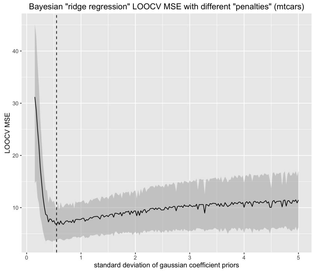
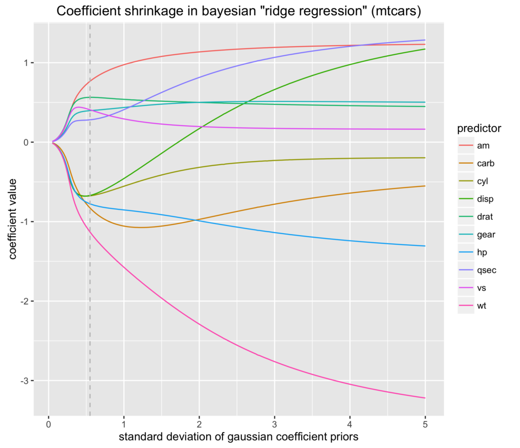
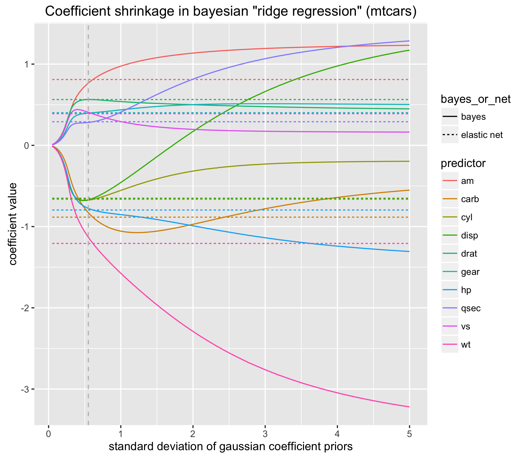
As it turns out, careful selection of the type and shape of our prior distributions with respect to the coefficients can mimic different types of frequentist linear model regularization. For ridge regression, we use normal priors of varying width.

Though it can be shown analytically that shifting the width of normal priors on the beta coefficients is equivalent to L2 penalized maximum likelihood estimation, the math is scary and hard to follow. In this post, we are going to be taking a computational approach to demonstrating the equivalence of the bayesian approach and ridge regression.

This post is going to be a part of a multi-post series investigating other bayesian approaches to linear model regularization including lasso regression facsimiles and hybrid approaches.

mtcars

We are going to be using the venerable mtcars dataset for this demonstration because (a) it’s multicollinearity and high number of potential predictors relative to its sample size lends itself fairly well to ridge regression, and (b) we used it in the TODO elastic net blog post :)

Before you lose interest… here! have a figure! An explanation will follow.

After scaling the predictor variables to be 0-centered and have a standard deviation of 1, I described a model predicting mpg using all available predictors and placed normal priors on the beta coefficients with a standard deviation for each value from 0.05 to 5 (by 0.025). To fit the model, instead of MCMC estimation via JAGS or Stan, I used quadratic approximation performed by the awesome rethinking package written by Richard McElreath written for his excellent book, Statistical Rethinking. Quadratic approximation uses an optimization algorithm to find the maximum a priori (MAP) point of the posterior distribution and approximates the rest of the posterior with a normal distribution about the MAP estimate. I use this method chiefly because as long as it took to run these simulations using quadratic approximation, it would have taken many orders of magnitude longer to use MCMC. Various spot checks confirmed that the quadratic approximation was comparable to the posterior as told by Stan.

As you can see from the figure, as the prior on the coefficients gets tighter, the model performance (as measured by the leave-one-out cross-validated mean squared error) improves—at least until the priors become too strong to be influenced sufficiently by the evidence. The ribbon about the MSE is the 95% credible interval (using a normal likelihood). I know, I know… it’s pretty damn wide.

The dashed vertical line is at the prior width that minimizes the LOOCV MSE. The minimum MSE is, for all practical purposes, identical to that of the highest performing ridge regression model using glmnet. This is good.

Another really fun thing to do with the results is to visualize the movement of the beta coefficient estimates and different penalties. The figure below depicts this. Again, the dashed vertical line is the highest performing prior width.

One last thing: we’ve heretofore only demonstrated that the bayesian approach can perform as well as the L2 penalized MLE… but it’s conceivable that it achieves this by finding a completely different coefficient vector. The figure below shows the same figure as above but I overlaid the coefficient estimates (for each predictor) of the top-performing glmnet model. These are shown as the dashed colored horizontal lines.

These results are pretty exciting! (if you’re the type to not get invited to parties). Notice that, at the highest performing prior width, the coefficients of the bayesian approach and the glmnet approach are virtually identical.

Sooooo, not only did the bayesian variety produce an equivalently generalizable model (as evinced by equivalent cross-validated MSEs) but also yielded a vector of beta coefficient estimates nearly identical to those estimated by glmnet. This suggests that both the bayesian approach and glmnet‘s approach, using different methods, regularize the model via the same underlying mechanism.

A drawback of the bayesian approach is that its solution takes many orders of magnitude more time to arrive at. Two advantages of the Bayesian approach are (a) the ability to study the posterior distributions of the coefficient estimates and ease of interpretation that they allows, and (b) the enhanced flexibility in model design and the ease by which you can, for example, swap out likelihood functions or construct more complicated hierarchal models.

If you are even the least bit interested in this, I urge you to look at the code (in this git repository) because (a) I worked really hard on it and, (b) it demonstrates cool use of meta-programming, parallelization, and progress bars… if I do say so myself :)

Known by those in-the-know, decorators are tools to make your python code beautiful, more concise, well-written, and elegant–but did you know you can use decorators to be a lazy programmer?!

I just recently whipped up a script that I’m using to help my expand and organize my photo library of my favorite pieces of art. This script that takes the URL of an art piece from artsy.net, downloads the image of the artwork and renames the downloaded file to follow a filename template (given as a CLI arg) based on the artist’s name, the title of the piece, and the date of completion. For example, if we wanted to download an image of the Fountain, and have the file automatically named: Marcel Duchamp - Fountain - 1917.jpg, one can use the following command:

1

python artsy-dl.py "https://www.artsy.net/artwork/marcel-duchamp-fountain-1" "%a - %t - %d"

because %a is automatically replaced with the artist’s name (that is extracted from the webpage), %t is automatically replaced with the title of the piece, and %d is the date of the piece.

In this post, I’ll be demonstrating the use of decorators to the end doing the bare minimum and how I saved myself from having to write tedious (but important) error-checking code. But before that, you, dear reader, have to be clear on what a decorator is. The section that follows is perhaps the greatest intro to decorators ever.

(If you are already familiar with decorators, you can skip to the section called “The problem”–though you may want to at least skim this section.)

What are decorators?

Here’s the skinny on Python decorators. Grokking decorators necessitates an intuitive understanding of three concepts:

• People often speak of functions as being “first-class citizens” in Python. By this they mean that functions are values that can be assigned to variables, returned from (other) functions, and passed as an argument to (still other) functions.
• When a function (we’ll call it outer) returns another function (we’ll call this inner), the inner function “closes over” (remembers) variables defined in the enclosing scope (outer‘s scope). If the returned function is stored in a variable and called at a later time, it still remembers the variable(s) from the enclosing scope—even if it is called long after the outer function finishes running and it’s variables otherwise lost. The inner function that is returned is known as a “closure”.
• A language that supports closures affords us the unique opportunity to easily add or modify the behavior of a function a by creating a function b that takes function a as an argument, and returns a function c which does something, and then calls function a. Function c can now be used in place of function a–it is essentially function a plus some extra functionality: it is a “decorated” version of function a.

In order to concretize these concepts, let’s see an example of a decorator complete with an illustration of the motivation behind creating it and the cognitive steps taken toward it’s finished state. Unlike some decorator tutorials, this lesson will not patronize you, dear reader, by designing a overly-simple decorator with no practical worth (it’s always been my thought that this pedagogical strategy most often backfires). Instead, we’ll create, you and I, a decorator of actual utility.

Suppose we wanted to time the execution of a function. Wanting something with a little more precision than a stopwatch, we decide to use the time module:

1
2
3
4
5
6
7
8
9

import time

def sleep_for_a_second():
    time.sleep(1)

start_time = time.time()
sleep_for_a_second()
end_time = time.time()
print("It took {0:.2f} seconds".format(end_time-start_time)) #> It took 1.00 seconds

This is ok, but if we want to time the execution of many different functions, this will result in a lot of repeated code. Being champions of the DRY principle, we decide it would be better to put this in a function:

1
2
3
4
5
6
7
8
9
10
11
12
13
14

def time_a_function(func):
    start_time = time.time()
    func()
    end_time = time.time()
    print("It took {0:.2f} seconds".format(end_time-start_time))

def sleep_for_a_second():
    time.sleep(1)

def sleep_for_two_seconds():
    time.sleep(2)

time_a_function(sleep_for_a_second) #> It took 1.00 seconds
time_a_function(sleep_for_two_seconds) #> It took 2.00 seconds

time_a_function is a function that takes the function we want to time as an argument.

We just timed two functions. Notice how we can now time an arbitrary number of functions with no extra code.

But there’s an issue with this approach. We’ve hitherto been timing functions that take no arguments. How would we time a function that takes one or more arguments?

1
2
3
4

def sleep_for_n_seconds(n):
    time.sleep(n)

time_a_function(sleep_for_n_seconds(5)) #> TypeError: 'NoneType' object is not callable

Nope. Before, we were passing the variable that holds the function to time_a_function, but the above incantation evaluates sleep_for_n_seconds(5), passes it’s None return value to time_a_function and because time_a_function can’t call it (because it’s not a function), we get an error. So how are we going to time sleep_for_n_seconds?

The solution is to make a function that takes a function that returns a function that takes an argument (n) and performs the function and times it and use the returned function in place of the original (whew!).

In other words:

1
2
3
4
5
6
7
8
9
10
11
12

def timer_decoration(func):
  def new_fn(n):
    start_time = time.time()
    func(n)
    end_time = time.time() print("It took {0:.2f} seconds".format(end_time-start_time))
  return new_fn

def sleep_for_n_seconds(n):
  time.sleep(n)

sleep_for_n_seconds = timer_decoration(sleep_for_n_seconds)
sleep_for_n_seconds(3) #> It took 3.01 seconds

Study this code carefully. You’ve just wrote a decorator. If you are confused it–as always with programming–helps if you type the code out yourself (no copy-and-pasting!) and play around with it.

Though it’s not terrible unwieldy otherwise, python gives us a nice elegant way to tag a particular function with a decorator so that the function is automatically decorated (i.e. doesn’t require us to replace the original function).

1
2
3
4
5
6
7

@timer_decoration
def sleep_for_n_seconds(n):
    time.sleep(n)

# now the reassignment of 'sleep_for_n_seconds' is unnecessary
sleep_for_n_seconds(3)
#> It took 3.00 seconds

But what happens if we try to decorate the original sleep_for_a_second function?

1
2
3
4
5
6

@timer_decoration
def sleep_for_a_second():
    time.sleep(1)

# sleep_for_a_second()
#> TypeError: new_fn() missing 1 required positional argument: 'n'

sleep_for_a_second is now expecting 1 argument :(. We can generalize our decorator to handle functions that take an arbitrary number of arguments with \*args and \*\*kargs…

1
2
3
4
5
6
7
8
9
10
11
12
13
14
15
16
17
18
19
20
21
22
23
24
25
26

def timer_decoration(func):
    def new_fn(*args, **kargs):
        start_time = time.time()
        func(*args, **kargs)
        end_time = time.time()
        print("It took {0:.2f} seconds".format(end_time-start_time))
    return new_fn

@timer_decoration
def sleep_for_n_seconds(n):
    time.sleep(n)

@timer_decoration
def sleep_for_a_second():
    time.sleep(1)

@timer_decoration
def sleep_for_k_seconds(k=1):
    time.sleep(k)

sleep_for_n_seconds(3)
#> It took 3.00 seconds
sleep_for_a_second()
#> It took 1.00 seconds
sleep_for_k_seconds(k=4)
#> It took 4.00 seconds

Ace!

Finally, let’s rewrite our decorator to support returning the return value of the decorated function.

1
2
3
4
5
6
7
8
9
10
11
12
13
14
15
16
17

def timer_decoration(func):
    def new_fn(*args, **kargs):
        start_time = time.time()
        ret_val = func(*args, **kargs)
        end_time = time.time()
        print("It took {0:.2f} seconds".format(end_time-start_time))
        return ret_val
    return new_fn

@timer_decoration
def sleep_for_a_second_p():
    time.sleep(1)
    return True

print(sleep_for_a_second_p())
#> It took 1.01 seconds
#> True

Note that our decorator is now generalized enough to be used with any function… no matter what it’s return type is… no matter what arguments it takes…

It doesn’t matter what the function is, the function’s behavior remains the same except now it is “decorated” with functionality that times it.

This is just one example of a decorator with obvious generalized utility. You can also use decorators to perform memoization, static-typing-like type enforcement of function signatures, automatically retry functions that failed, and simulate non-strict evaluation.

The problem

To review, I wrote a script that takes the URL of an artwork on artsy.net, downloads the image, and then names the file in accordance with a user-supplied format string that uses info about the artwork. With the help of the requests, lxml, and wget modules, a script to do this can be coded relatively quickly. The problem, though–which is common for scripts that talk to the web that don’t do error-checking–is that the script is brittle. Without error-checking, any malformed URL, network interruption, invalid output path, or weird edge case like an artwork without a title, will result in an unsightly error message and lengthy stack trace. Besides being aesthetically objectionable, if anyone else is using your script, you will look like an incompetent software engineer. So you have to bite the bullet and error-check.

The problem with error-checking is

• If all possible errors are checked for separately and individually and handled appropriately (this is good practice), it will result in code often many times longer than the original code. Only a small fraction of the code will be the actual interesting logic of the program–most of it will now be mindless conditionals.
• It’s difficult for someone without training (me) to anticipate every possible error.
• It takes a lot of work and I’m lazy

So my usual M.O. is to wrap each component in a try/except block (with no specificity in the exception), print an error message, and terminate execution…

1
2
3
4

try:
    <brittle code>
except:
    sys.exit("<brittle code> broke")

Except I don’t even do that. Instead of wrapping each component in a try/except with its own error message, I just wind up try/excepting main once. This cuts down typing and carpal tunnel is a real thing…

1
2
3
4
5
6
7

def main():
    <literally everything>

try:
    main()
except:
    sys.exit("whoopsie daisy")

Decorators to the rescue

Okkkaaaayyyyy… if we absolutely must do some modicum of error checking around each component (so the user has some kind of clue as to why it the script’s usage failed) we can write a decorator to do this for us. The following is an excerpt of the script as of commit d6be4956543:

1
2
3
4
5
6
7
8
9
10
11
12
13
14
15
16
17
18
19
20
21
22
23
24
25

...
# the decorator
def cop_out(f):
    def inner(*args, **kargs):
        try:
            return f(*args, **kargs)
        except:
            sys.exit("\nThe function <{}> failed\n".format(f.__name__))
    return inner

@cop_out
def get_command_line_arguments():
    return sys.argv[1], sys.argv[2]

@cop_out
def download_webpage(url):
    r = requests.get(url)
    if r.status_code != 200:
        raise Exception
    return r

@cop_out
def parse_webpage(requests_object):
    return lxml.html.fromstring(requests_object.text)
....

Note how we use f.__name__ to get the name of the function that was decorated. This allows us to add the support for specialized (at the function level, at least) error messages for free!

Now, if the user calls the script with too few arguments, the program will print The function <get_command_line_arguments> failed. If you give it a real URL but not to an artsy.net artwork, it’ll say The function <extract_artist_name_from_webpage> failed. If you give it a made-up URL, it’ll say The function <download_webpage> failed, etc…

Sure, beyond the function level, you don’t know why it failed, but anything is better than nothing and your users shouldn’t be so bossy and entitled.

But one more thing… if you looked at the code, you’ll notice that my function names are descriptive… maybe too long and descriptive. The use of prose-like descriptive function names (certainly by the standards of Haskell programmers) was no accident. Although it may seem like an uncharacteristically diligent and conscientious decision on my part, it was actually to facilitate further laziness. Consider the following tweak to the decorator:

1
2
3
4
5
6
7
8

def cop_out(f):
    def inner(*args, **kargs):
        try:
            return f(*args, **kargs)
        except:
            message = f.__name__.replace("_", " ")
            sys.exit("\nFailed to {}\n".format(message))
    return inner

Consider how this generates error messages that appear to individualized…

1
2
3
4
5
6
7
8
9
10

$ python artsy-dl.py "https://www.artsy.net/artwork/jean-michel-basquiat-untitled-33211237"
Failed to get command line arguments

$ python3.4 artsy-dl.py "https://www.artsy.net/artwork/jean-michel-BAHHSKIIIAAHT-untitled-33211237"
                        "%a/%t - %d"
Failed to download webpage

$ python2.7 artsy-dl.py "https://www.artsy.net/artist/jean-michel-basquiat"
                         "%a/%t - %d"
Failed to extract artist name from webpage

So there you have it! Decorators can be used for legitimate, elegant solutions but can also be employed–virtually for free–to give the illusion that you are a caring software engineer and meticulous with your error checking.

PS

If you’re a potential employer or client, I’m just kidding–I’m very diligent about error checking. This piece is satire. I promise.

As regular readers of this blog may be aware, one of my favorite activities is marshaling the skills that I use as a computational scientist to study the humanities. For example, in a previous post, we saw how principles from phylogenetic systematics helped textual critics reconstruct the original manuscript for “The Canterbury Tales”; in another, we deployed techniques first used to study physics to the end of fooling vineyards into retweeting fake, computer-generated wine reviews.

For this post, I used both tools from computational linguistics and some good-old-fashioned data wrangling (web-scraping, parsing texts, etc…) to create a custom-fit Spanish verb study guide.

The problems

Problem #1

Although foreign language immersion is the almost certainly the best learning path for most types of foreign language learners, no reasonable student without an lavish budget for traveling can expect to get by without having to do some rote memorization. In the context of Spanish verbs, this either means unguided memorization of a dictionary or consultation of a list of the most commonly used Spanish verbs. But, even if you could trust that the most-popular-verbs list was compiled in a principled manner, there are vast regional and sub-culture-specific variations in verb frequency. For example, the verb coger means “to take” in Spain but in Central America it’s… it’s a… pretty vulgar verb. It stands to reason that there are pretty enormous differences in this verb’s popularity across regions, contexts, and registers. Depending on which region’s dialect you prioritize familiarity with, and depending on how raggle-taggle the people you intend to roll with are—or the media you intend to consume—a one-size-fits-all verb list might let you down.

Problem #2

English isn’t a very inflective language—the tense (or person, mood, aspect, etc…) is largely determined, not through verb conjugation, but via periphrasis, the use of personal pronouns, and other auxiliary words. This is in stark comparison to Spanish, a highly-inflective, relatively synthetic language where the verb’s conjugation betrays its tense, person, mood, and aspect—all in one word! This linguistic elegance is a learning obstacle, since one verb might be written in a little under 60 different ways (6 persons * (4 tenses in the indicative mood + 3 tenses in the subjunctive mood + 1 imperative mood)). This pedagogical nightmare is partially allayed by careful prioritization of some tenses and moods, over others—at least initially. For example, a Spanish-language learner almost always learns the commonly-used and versatile present indicative tense first. But beyond the next few obvious choices, the order in which these tenses should be prioritized is not clear and (probably) dependent on how and where you expect to use and consume the language. Further complicating things, there are entire persons (here’s looking to you, vosotros) that are very uncommon in most Spanish-speaking countries.

The solution

The solution to this problem is to create a personal corpus of Spanish text, containing examples of the types of text you expect to consume and produce. Then, the verbs need to be identified, have their mood, tense, and person recorded, and converted into infinitive form (for frequency tabulation). The relative frequencies of the persons, mood, and tenses—as well as the frequencies of the verbs (in infinitive form)—will inform the creation of a Spanish verb study guide specifically catered to type of linguistic variety the learner intends to employ. Whether the learner’s primary interest in learning Spanish is to be able to bond with a new family member over their love of Mexican telenovelas or to read and understand Don Quixote in its entirety, this approach will hasten the learner’s sense of accomplishment with respect to cookie-cutter verb study guides, increase learner satisfaction, and increase the likelihood of the learner actually achieving language mastery. I mean, as a learner myself, I would be discouraged if I felt like the main payoff of studying Spanish is to read and understand books that are very obviously juvenile or primary meant for pedagogical purposes. I want to read Márquez and I want to read him now!

The corpus

For my particular corpus, I chose a whole mess of books (most of which I’ve read—and loved—in English) that I’m interested in reading in the original language. These include Rayuelas and Final De Juego by Julio Cortázar (my favorite short story writer), Cien Años De Soledad by Gabriel García Márquez (generally considered to be a masterpiece), Darios de Motocicleta by Che Guevara, Ficciones by Jorge Luis Borges, and La Cuidad De Las Bestias by Isabel Allende. These texts were obtained electronically—legitimately!—and I used various ad-hoc regexes to remove formatting and conversion-from-PDF-to-text) artifacts.

My interest in Spanish isn’t only for consuming literature, though; I wanted to include other sources of text, like movie scripts (I planned on Lo Que le Pasó a Santiago, generally considered to be one of the best Puerto Rican films), but I couldn’t find the script online. I also wanted to include the lyrics to my favorite Spanish-language bands (Soda Stereo, El Ultimo Vecíno, Décima Víctima, Caifenes, Shakira, Millie Quezada, …) but the tool I used to identify the verbs in the corpus often choked on these texts. Why, you ask?…

Parts-of-speech tagging

references are at the bottom of the post

Parts-of-speech tagging (hereafter, ‘POS tagging’) is when you go through a text and, for each word, identify the which part of speech (verb, noun, adjective, etc…) the word functions as.

This is a non-trivial task because the same word can function as different parts-of-speech depending on the context. Take the following sentence, for example, which is an expanded and modified version of a sentence that is used as an example in this video

Fruit flies like bananas

So, taken individually, all words in this sentence can function as multiple parts of speech. Take “like” for instance; it can be a noun (“my status got mad likes“), a verb (“I like your status“), a quotative (“I was like, ‘I enjoyed your status‘“), conjunction (_“I updated my status like the world depended on it_”), a preposition (“I wrote my status like Nathaniel Hawthorne“). Depending on how colloquial the text in question is, “like” can even be used as a discourse marker (“I’m, like, scared of ghosts, Scoob“). As a standalone word, “like” can serve the purpose of 6 different parts of speech.

But even looking at the entire sentence as a whole, the parts-of-speech for each word is ambiguous.

Concretely, the sentence can be interpreted as (a) “fruit flies (noun) like (verb) bananas (noun)”, (b) “fruit (noun) flies (verb) like (preposition) bananas (noun) [do]”, or even (c) “fruit (noun) flies (verb) like (conjunction(?)) bananas (adjective)”—using the colloquial meaning of the word bananas meaning “crazy”.

Note that the POS tag for one word is conditional on the POS tags of other words: whether flies is a noun or a verb affects whether bananas is interpretable as a adjective.

Because this task isn’t easy, this job used to be left to humans to perform. Now, various techniques allow for this to be done programmatically to a high degree of accuracy. We’ll go through a few of them, ending with the sophisticated method employed by the POS tagger that we will be using, the Stanford Parts-of-speech tagger.

Unigram tagging

A training corpus with the POS tags for each word is read and, for each unique word, the number of times it is used as one of the various parts of speech is tallied. When a word is encountered in untagged text, the tagger chooses the part-of-speech that the word is most commonly used as in the training text. If the word encountered was not in the training text at all, it defaults to a noun. Somehow, this context-free elementary method can yield accuracies of 90%-94% (Brill & Wu, 1998). When Brill and Wu used this method with/on the famous Penn Treebank Wall Street Journal corpus with a 80%/20% training/testing split, it achieved 93.3% accuracy.

n-gram tagging

Using an n-gram model, the tag of a particular word is assumed to be conditionally dependent on the tag of the preceding n-1 words. For example, in a bigram model, the tag of the current word is guessed from the current word, and the tag of the previous word. A trigram model uses tag information from the previous two words, in concert with the conditional probability of a particular tag given a certain word. The unigram tagger is a special case of the _n_-gram tagger where n is 1. It’s not hard to see that _n_-gram tagging will offer an enormous accuracy improvement.

If this reminds you of the Markov chains that we made use of in the previous post on computer-generating wine reviews, then you have a good eye. N-gram tagging is a type of Hidden Markov Model (HMM). What makes HMMs different than simple Markov models is that the states themselves (the POS tags) are not directly observable; the observable portion of each state are the actual words—and the words are only a probabilistic function of the state.

In addition to testing a unigram model, Brill and Wu also tested this technique’s ability on the WSJ corpus. In particular, they used a trigram tagger—with a twist. Weischedel, Ralph, et al (1993) noted that the suffix of a word (-ed, -s, -ing, -ion, -ly, etc…) strongly influenced the probability that the word served as a particular part of speech. When this information was wielded to help classify unknown words, it greatly improved accuracy outcomes. When Brill and Wu used this method with a trigram tagger against the WSJ corpus, the technique yielded an 96.4% accuracy rate.

Maximum Entropy models

Maximum Entropy models are a lot like—insofar as they are equivalent to—multinomial logistic regression models that attempt to model the probability of a given tag class given various predictor variables, or features. Maximum entropy models can use features such as the current word, the previous word, the previous word’s tag, etc…—like would a HMM—but also features like whether the word contains a number, whether the word is capitalized, etc… An optimization algorithm called Generalized Iterative Scaling selects the feature weights that maximize the likelihood function.

Ratnaparkhi (1996) tested a straightforward maximum entropy model on the WSJ corpus and noted that it yielded an accuracy of 96.6%. Four years after that, Toutanova et al. (2000) published a paper in which they show that by adding additional features like whether the word is capitalized and in the middle of a sentence and non-local features that look 8 words back for a modal verb (for disambiguating base form verbs and non-3rd person singular present verbs) they can achieve a WSJ accuracy of 96.8%. This is the benefit of the Maximum Entropy model approach—you can arbitrarily add features (within reason) without necessarily knowing how those features contribute the the probabilities of tag outputs.

Three years after that, Toutanova et al. (2003) achieved a 97.2% accuracy rate on the WSJ corpus by (a) adding features for the words following the word currently being tagged, and (b) using regularization to combat overfitting as a result of using many features—many of which probably only weakly contribute information of the probability of the current word’s tag class. Their regularization technique involved placing a zero-centered Gaussian prior on the feature weights and is mathematically tantamount to the L2 regularization that we saw in this previous blog post. This state-of-the-art tagger is the one on which the Stanford tagger we use is based.

There is another famous type of POS tagger called Transformation-Based tagger. In contrast to all the others that were mentioned above, this is not a probabilistic/stochastic model and is, instead, based on rules and knowledge. I won’t describe it here because it’s very different and this post is already too long but I should mention that it can score a 96.6% on the on WSJ corpus (Brill et al., 1998).

The procedure

These steps assume a POSIX compliant system and some command-line proficiency

The filenames are links and you can find a repo with all the code here

• Downloaded full version of the Stanford Parts-of-speech tagger
• Ran the tagger on the text, put each tag on a separate line, and filtered for verbs only. The parts-of-speech were identified using this tagset. As you can see, the verbs all start with the letter “v”. This can be achieved by the following incantation:

1

./stanford-postagger.sh models/spanish.tagger THE_BOOK.txt perl -pe 's/ /\\n/g' grep '_v' > tmp

If this causes you problems, you might want to try to give the tagger (which runs in multicore!) more memory; try adding -Xmx2048M as a argument in the java command in ./stanford-postagger.sh—this will give it 2GBs to work with.

• For each work, I ran this.py on it, which parsed the stanford tag and made it in nice tab delimited format:

1

./stanford-output-to-nice-tsv.py < tmp > ./output-verbs/THE_BOOK.txt

• Catted all of them together into all.txt–a monstrous text file with 84,437 words that the tagger interpreted as verbs:

1

cat rayuelas.txt final-de-juego.txt darios-de-motocicleta.txt cien-anos-de-soledad.txt ficciones.txt la-cuidad-de-las-bestias.txt > all.txt

Now we need to get the infinitives, but in order to prioritize which we should get the infinitives for, and not have to repeat conjugated verbs, we need to get the uniques…

• So I ran

1

cat all.txt perl -pe 's/(.+?)\\t.\*/\\1/g' > all-verbs.txt

to get a list of only verbs (no mood or tense)

• I wanted to get a list of unique verbs sorted by the number of occurrences; this would normally be a job for the sort uniq -c. Desafortunademente, this command fails. It turns out that unicode can represent (for example) habría in at least two different ways. For this reason, we have to use the python script process-all-verbs.py which uses the unicodedata module to normalize the verbs and then count them.

1

./process-all-verbs.py tee all-verbs-count.txt

Ok, now were ready to get infinitive forms for these verbs. We are going to do this by programmatically making request to translate the word to the (excellent) website Span¡shD!ct.com. What we want can be extracted from the returned HTML via CSS selectors.

• get-infinitives.py goes through each line of all-verbs-count.txt and constructs the url to query the website with. It then uses the CSS selector “.mismatch” for information about the verb.

In the best case scenario, it says something like “___“ is the ____ form of _____ in the ____“. Sometimes, there’s more than one possible person or tense so it says “____ represents different conjugations of the verb _____“

In either case, we get the infinitive. If it fails, we record it and move on. It waits between 1 and 2 seconds between each verb. After every 20, it dumps the JSON so that in case something bad happens I could just load the intermediate results and restart.

• You can see that the SpanishDict infinitive conversion systematically failed for certain words. For example, it interpreted inflected verbs like he, dice, and era as English words to translate, not Spanish words to provide information for. In other cases, it interpreted a verb’s past participle (aburrir -> aburrido (“to bore”)) as an adjective (“boring”). I manually filled in many of the ones that failed using equal parts regex and black magic. This went into finished-supplemented.json.
• Finally, we need to inner join all.txtto the information infinished-supplemented.json. The combine.py script does this:

1

./combine.py tee tagged-plus-infinitives.txt [/code]

The tab-delimited tagged-plus-infinitives.txt in now ready to be consumed for analysis.

Some numbers

• Rayuelas - 203,197 words - 29,882 verbs Final de juego - 54,303 words - 8,160 verbs Darios de Motocicleta - 53,804 words - 6,557 verbs Cien Años de Soledad - 15,4381 words - 20,987 verbs Ficciones - 48,845 words - 5,769 verbs La Cuidad De Las Bestias - 94,075 words - 13,082 verbs
• There were 84,437 words that the tagger identified as verbs in all.
• There were 13,972 unique conjugated verbs.
• After the first try with SpanishDict, for only 6,852 verbs did we have the infinitives. This greatly increased with the black magic alluded to in the previous section.
• I went from 84,437 to 71,378 verbs when I inner joined with the verbs that I was able to find infinitives for.

The results

Proportion of Spanish verb moods and tenses in corpus

The results were rather fascinating.

These were the 14 most common conjugated verbs:

(you can see the full spreadsheet here)

With this information alone, this whole endeavor was worth it. Sure, most of the verbs in this list aren’t that much of a surprise, but there are two pieces of information that could prove really helpful to me. The first is that 4 verbs in the top 15 are forms of the verb haber (“to have”)—including the very first one, which accounts for 3.6% of all conjugated verbs in the corpus. This is a verb that I was, heretofore, relatively unfamiliar with.

In contrast to tener (which also means “to have”), haber is often used as an auxiliary verb as it would in such english sentences as “I have to go to the dentist”, “I had all but lost it” (past perfect tense), “there is a freeze-up coming”. Because of it’s ubiquitous usage as an auxiliary word (like its being used in all sentences in the perfect mood), I should get more familiar with this verb and its conjugations if I ever hope to read these works of literature.

The second important piece of information for me was that a majority of the verbs in the top 14 were in the imperfect tense (a type of past tense). Now, I think I may have been concentrating too much on the preterite tense (another past tense) in comparison. Next, these were the 14 most common verbs when put into infinitive form:

(you can see the full spreadsheet here)

To me, there wasn’t really anything unexpected here except for maybe pasar (to happen) and parecer (to seem), which I was, up until this point—relatively unfamiliar with in spite of the fact that they are used in a number of frequently spoken expressions like ¿Que pasó? (“What happened?”) and ¿Que te parece? (~”What do you think?”).

Finally, figure 1 is a plot which depicts the proportions in which each mood and tense occur. The large vertical bars show the relative proportions of each mood (I count the Infinitive, Gerund, and Participle as moods) in descending order; they are Indicative (65%), Infinitive (20%), Subjunctive (4%), Participle (4%), Gerund (3%), and Imperative (1%). Each vertical bar is further broken down by the proportion of each tense within that mood (sorted, with the most frequently used on the bottom. For example, the present tense is the most common tense in the indicative mood and accounts for 26% of all mood/tense pairs. The Infinitive, Participle, and Imperative moods (to the extent that there are actually moods) have only one tense (to the extent that they can be said to have tenses).

These results were most surprising to me; for one, I was (again) reminded that I should probably hold nailing down the imperfect tense with as much or more importance as I do with the preterite tense. Second, I was surprised that usage of the future tense was far eclipsed by gerund, participle, and both subjective tenses—in spite of the fact that I use it quite often in my texts to my friends and my internal monologue. Of course, this—and other insights—may just be artifacts of the particular body of literature I chose for my corpus (see next section).

Limitations:

Although this was a wildly fun project that yielded interesting and extremely practical insights, there are a number of important caveats to be aware of when interpreting these results.

First is a generalizability issue; the results indicate the verb popularity and mood/tense breakdowns for just 6 pieces of Spanish literature. Because of this, the corpus is heavily dominated by the writing style of the included authors—at least some of whom have a very idiosyncratic writing style. Additionally, as with most literature, all of the non-short-stories in my corpus were told in the past tense (usually by a third person omniscient narrator). This past tense bias is very clearly non-representative of everyday spoken Spanish (of course, it was never meant to be representative of that). This problem could have been, at least partially, alleviated via the inclusion of more prosaic Spanish from movie scripts and blogs—if only they POS tagged correctly!!

Speaking of tagging correctly, the second issue is one of the correctness of the POS tags. The best POS taggers (Stanford is certainly one) can, at best, achieve an accuracy of 97%. Although this is an incredible feat of computational linguistics and the product of many many years of research, it is important to put this in the proper perspective. Recall that the rudimentary unigram tagger can achieve a 90%-94% accuracy rate (b) the 97% accuracy rate decreases as the testing corpus diverges in style from the training corpus. Especially because of Cortázar—who (at least in English translations) employs highly unusual sentence structure and often straight-up grammatically-incorrect non-human-parsable sentences—this fact must be kept in mind; unless the Spanish model that comes with Stanford was trained with Surrealist literature (it wasn’t!), tag accuracy will suffer.

References

Brill, Eric, and Jun Wu. “Classifier combination for improved lexical disambiguation.” Proceedings of the 36th Annual Meeting of the Association for Computational Linguistics and 17th International Conference on Computational Linguistics-Volume 1. Association for Computational Linguistics, 1998.

Ratnaparkhi, Adwait. “A maximum entropy model for part-of-speech tagging.” Proceedings of the conference on empirical methods in natural language processing. Vol. 1. 1996.

Toutanova, Kristina, and Christopher D. Manning. “Enriching the knowledge sources used in a maximum entropy part-of-speech tagger.” Proceedings of the 2000 Joint SIGDAT conference on Empirical methods in natural language processing and very large corpora: held in conjunction with the 38th Annual Meeting of the Association for Computational Linguistics-Volume 13. Association for Computational Linguistics, 2000.

Toutanova, Kristina, et al. “Feature-rich part-of-speech tagging with a cyclic dependency network.” Proceedings of the 2003 Conference of the North American Chapter of the Association for Computational Linguistics on Human Language Technology-Volume 1. Association for Computational Linguistics, 2003.

Weischedel, Ralph, et al. “Coping with ambiguity and unknown words through probabilistic models.” Computational linguistics 19.2 (1993): 361-382.

In the chapter “Sources of Data” I show how to consume web data of different formats in R. The motivating example is to build a simple recommendation system that uses user-supplied “tags” (genres/labels) submitted to Last.fm and MusicBrainz to quantify musical artist “similarity”. The example in the book stops at the construction and sorting of the similarity matrix but, in this post, we’re going to make a really fly D3 visualization of the musical similarity network and provide recommendations in the tooltips. The code, including the Javascript and HTML, I used for this post was hastily thrown into a git repo and is available here. If you’re uninterested in the detailed methodology, I suggest you skip to the section labeled “Outcome”.

Methodology

Although in the book tags from both Last.fm and MusicBrainz are used, we’ll just be using Last.fm here. (In additional contrast to the book, the code here is, as you might imagine, substantially faster-paced.)

The first step is to make a character vector of all the artists that you’d like to be included. If you were building a real system, you’d probably want all Last.fm artists. Since we’re not, I just used 70 of my most played artists on my Last.fm. Since I got the list straight from the source, I didn’t have to worry that any of the API requests would return “No Artist Found”.

The following is a function that takes an artist and returns the properly formatted Last.fm API call to get the tags in JSON format.

1
2
3
4
5

create_artist_query_url_lfm <- function(artist_name){
  prefix <- "http://ws.audioscrobbler.com/2.0/?method=artist.gettoptags&artist="
  postfix <- "&api_key=c2e57923a25c03f3d8b317b3c8622b43&format=json"
  encoded_artist <- URLencode(artist_name) return(paste0(prefix, encoded_artist, postfix))
}

This is an example of the JSON payload from my favorite merengue artist.

We only want the tag names–curiously, attempts to factor in degree of tag fit (the “count” attribute) resulted in (what I interpreted as) substantially poorer recommendations.

The following is a function that will return a vector of all the tags.

1
2
3
4
5
6
7

library(jsonlite)

get_tag_frame_lfm <- function(an_artist){
  print(paste0("Attempting to fetch: ", an_artist))
  artist_url <- create_artist_query_url_lfm(an_artist)
  json <- fromJSON(artist_url) return(as.vector(json$toptags$tag[,"name"]))
}

Since the above function is referentially transparent, and it involves using resources that aren’t yours, it’s a good idea to memoize the function so that if you (accidentally or otherwise) call the function with the same artist, the function will return the cached result instead of making the web request again. This can be achieved quite easily with the memoise package.

1
2
3

library(memoise)

mem_get_tag_frame_lfm <- memoise(get_tag_frame_lfm)

To get the tags from all the artists in our custom ARTIST_LIST vector..

1
2

artists_tags <- sapply(ARTIST_LIST, mem_get_tag_frame_lfm)
names(artists_tags) <- ARTIST_LIST

To get a list of all pairs of artists to compute the similarity for, we can use the combn function to create a 2 by 2,415 character matrix of all possible combinations (choose 2). Let’s get that into a 2,415 by 2 data.frame with the name “artist1” and “artist2”…

1
2
3

cmbs <- combn(ARTIST_LIST, 2)
comparisons <- data.frame(t(cmbs))
names(comparisons) <- c("artist1", "artist2")

The similarity metric we’ll be using is simple as all get-out: the Jaccard index. Assuming we put the tags from both artists into two sets, it is the cardinality of the sets’ intersection divided by the sets’ union…

1
2
3
4
5
6
7

jaccard_index <- function(tags1, tags2){
  length(intersect(tags1, tags2))/length(union(tags1, tags2))
}

comparisons$similarity <- apply(comparisons, 1, function(arow){
  jaccard_index(artists_tags[[unlist(arow[1])]], artists_tags[[unlist(arow[2])]])
})

Now we’ve added a new column to our previously 2,415 by 2 data.frame, “similarity” that contains the Jaccard index.

Our D3 visualization expects a JSON with two top level attributes: “nodes” and “links”. The “nodes” attribute is an array of x number of 5 key-value pairs (where x is the number of nodes). The 5 keys are “name” (the name of the artist) “group” (a number that affects the coloring of the node in the visualization that we will be setting to “1”), and “first”, “second”, and “third”, which are the top 3 most similar artists and will serve as the recommendations that pop-up in a tool-tip when you mouse over an artist node in the visualization.

This is some code to get the top 3 most similar artists. It takes the 2,415 by 3 comparisons data.frame, the number of “most similar artists” to return, an artist, and an arbitrary threshold for “similar-ness” as arguments. Any similarity below this threshold will not be considered a viable recommendation.

1
2
3
4
5
6
7
8
9
10
11

library(dplyr)

get_top_n <- function(comparisons, N, artist, threshold){
  comparisons %<>%
    filter(artist1==artist artist2==artist) %>%
    arrange(desc(similarity))
  other_artist <- ifelse(comparisons$similarity>threshold,
                    ifelse(comparisons$artist1==artist,
                           comparisons$artist2, comparisons$artist1), "None")
  return(other_artist[1:N])
}

The inner ifelse clause has to handle the fact that the “similar” artist can be in the first column or the second column. The outer ifelse returns “None” for every similarity value that is not above the threshold.

Let’s make the data.frame that will serve as the “nodes” attribute in the final JSON…

1
2
3
4
5
6

nodes <- sapply(ARTIST_LIST, function(x) get_top_n(comparisons, 3, x, 0.25))
nodes <- data.frame(t(nodes))
names(nodes) <- c("first", "second", "third")
nodes$name <- row.names(nodes)
row.names(nodes) <- NULL
nodes$group <- 1

For the other top-level JSON attribute, “links”, we need an array of y number of 5 key-value pairs where y is the number of sufficiently strong similarities between the artists. The 5 keys are “node1” (the name of the first artist), “source” (the 0-indexed index of the artist with respect to the array in the “nodes” attribute), “node2” (the name of the second artist), “target” (the index of the second artist) and “weight”, which is the degree of similarity between the two artists; this will translate into thicker “edges” in the similarity graph.

1
2
3
4
5
6
7
8
9
10
11

# find the 0-indexed index

lookup_number <- function(name)
  which(name==ARTIST_LIST)-1

strong_links <- comparisons %>%
  filter(similarity > 0.25) %>%
  rename(node1 = artist1, node2 = artist2, weight=similarity)

strong_links$source <- sapply(strong_links$node1, lookup_number)
strong_links$target <- sapply(strong_links$node2, lookup_number)

Finally, we can create the properly formatted JSON and send it to the file “artists.json” thusly…

1
2
3
4

object <- list("nodes"=nodes, "links"=strong_links)
sink("artists.json")
toJSON(object, dataframe="rows", pretty=TRUE)
sink()

Outcome

Using “artists.json” and the “index.html” that can be found here, the similarity graph looks a little like this. (Make sure you scroll to see the whole thing.)

For illustrative purposes, I pre-labeled the artists’ “group” with labels that correspond to what I view as the artist’s primary genre. This is why the nodes in the linked visualization have different colors. Note that, independently, the genres that I indicated tend to cluster together in the network. For example, Reggae (light green), Hip-Hop (green), and Punk (orange) all form almost completely connected graphs, though unconnected to each other (disjoint subgraphs). Indie rock (blue), post-punk (light blue) and classic rock (light orange) together form a rather tightly-connected subgraph. Curiously, the Sex Pistols (that I labeled “Punk”) are not part of the Punk cluster but part of the Indie-rock/post-punk/classic-rock component. There are three orphan nodes (no edges), “Johann Sebastian Bach”, “P:ano“, and “No Kids“. Bach is orphaned because he’s the only Baroque artist in my top 70 artists :( –P:ano and No Kids are obscure… you’ve probably never heard of them.

The recommendations, prima facie, appear to be on point. For example, without direct knowledge of association, “KRS-One” recommends “Boogie Down Productions” (the group that KRS-One comes from) most highly. Similarly, “The Smiths” and “Morrissey” recommend each other, and “De La Soul” and “A Tribe Called Quest” (part of a positive, Afrocentric hip-hop collective known as the Native Tongues together with Queen Latifah, et al.) recommend each other.

Appropriately, Joy Division and New Order, whose Jaccard index of band members is 0.6 but whose music style is somewhat distinct, don’t recommend each other. Lastly, subgenred artists appear to recommend other artists in the subgenre. For example, goth band “The Sisters of Mercy” appropriately recommends other goth-esque bands “Bauhaus”, “And Also The Trees”, and “Joy Division”.

Afterword

Using this similarity measure to drive recommendations seems successful. It should be noted, though, that my ability to assess the effectiveness of using the Jaccard index as the sole arbiter of musical similarity is hampered; judging an algorithm on the basis that the system recommends other bands that I necessarily like is prejudicial, to say the least.

This stands even if the system makes good theoretical sense. This still stands even if the system, quite independently, indicates that associated acts—that are objectively and incontrovertibly similar—are good recommendations.

This raises a larger question on how to accurately measure the effectiveness of recommender systems; do you tell people what they want to hear, or do you pledge allegiance to a particular theoretical interpretation of similarity? If it’s the latter, how do you iterate and improve the system? If it’s the former, is your only criterion for success positive user-provided feedback?

Lasso regression is a related regularization method. Instead of using the L2 norm, though, it penalizes the L1 norm (manhattan distance) of the coefficient vector.

Because it uses the L1 norm, some of the coefficients will shrink to zero while lambda increases. A similar effect would be achieved in Bayesian linear regression using a Laplacian prior (strongly peaked at zero) on each of the beta coefficients. Because some of the coefficients shrink to zero, the lasso doubles as a crackerjack feature selection technique in addition to a solid shrinkage method. This property gives it a leg up on ridge regression. On the other hand, the lasso will occasionally achieve poor results when there’s a high degree of collinearity in the features and ridge regression will perform better. Further, the L1 norm is underdetermined when the number of predictors exceeds the number of observations while ridge regression can handle this.

Elastic net regression is a hybrid approach that blends both penalization of the L2 and L1 norms. Specifically, elastic net regression minimizes the following…

the hyper-parameter is between 0 and 1 and controls how much L2 or L1 penalization is used (0 is ridge, 1 is lasso).

The usual approach to optimizing the lambda hyper-parameter is through cross-validation—by minimizing the cross-validated mean squared prediction error—but in elastic net regression, the optimal lambda hyper-parameter also depends upon and is heavily dependent on the alpha hyper-parameter (hyper-hyper-parameter?).

This blog post takes a cross-validated approach that uses grid search to find the optimal alpha hyper-parameter while also optimizing the lambda hyper-parameter for three different data sets. I also compare the performances against the stepwise regression and showcase some of the dangers of using stepwise feature selection.

mtcars

In this example, I try to predict “miles per gallon” from the other available attributes. The design matrix has 32 observations and 10 predictors and there is a high degree of collinearity (as measured by the variance inflation factors).

The left panel above shows the leave-one-out cross validation (LOOCV) mean squared error of the model with the optimal lambda (as determined again by LOOCV) for each alpha parameter from 0 to 1. This panel indicates that if our objective is to purely minimize MSE (with no regard for model complexity) than pure ridge regression outperforms any blended elastic-net model. This is probably because of the substantial collinearity. Interestingly, the lasso outperforms blended elastic net models that weight the lasso heavily.

The right panel puts things in perspective by plotting the LOOCV MSEs along with the MSE of the “kitchen sink” regression (the blue line) that includes all features in the model. As you can see, any degree of regularization offers a substantial improvement in model generalizability.

It is also plotted with two estimates of the MSE for models that blindly use the coefficients from automated bi-directional stepwise regression. The first uses the features selected by performing the stepwise procedure on the whole dataset and then assesses the model performance (the red line). The second estimate uses the step procedure and resulting features on only the training set for each fold of the cross validations. This is the estimate without the subtle but treacherous “knowledge leaking” eloquently described in this plot post. This should be considered the more correct assessment of the model. As you can see, if we weren’t careful about interpreting the stepwise regression, we would have gotten an incredibly inflated and inaccurate view of the model performance.

Forest Fires

The second example uses a very-difficult-to-model dataset from University of California, Irvine machine learning repository. The task is to predict the burnt area from a forest fire given 11 predictors. It has 517 observations. Further, there is a relatively low degree of collinearity between predictors.

Again, highest performing model is the pure ridge regression. This time, the performance asymptotes as the alpha hyper-parameter increases. The variability in the MSE estimates is due to the fact that I didn’t use LOOCV and used 400-k CV instead because I’m impatient.

As with the last example, the properly measured stepwise regression performance isn’t so great, and the kitchen sink model outperforms it. However, in contrast to the previous example, there was a lot less variability in the selected features across folds—this is probably because of the significantly larger number of observations.

“QuickStartExample”

This dataset is a contrived one that is included with the excellent glmnet package (the one I’m using for the elastic net regression). This dataset has a relatively low degree of collinearity, has 20 features and 100 observations. I have no idea how the package authors created this dataset.

Finally, an example where the lasso outperforms ridge regression! I think this is because the dataset was specifically manufactured to have a small number of genuine predictors with large effects (as opposed to many weak predictors).

Interestingly, stepwise progression far outperforms both—probably for the very same reason. From fold to fold, there was virtually no variation in the features that the stepwise method automatically chose.

Conclusion

So, there you have it. Elastic net regression is awesome because it can perform at worst as good as the lasso or ridge and—though it didn’t on these examples—can sometimes substantially outperform both.

Also, be careful with step-wise feature selection!

PS: If, for some reason, you are interested in the R code I used to run these simulations, you can find it on this GitHub Gist.

The example problem is to find the mean distance between every airport in the United States. This silly example was chosen because it exhibits polynomial growth in running time as a function of the number of airports and, thus, quickly becomes intractable without sampling. It is also easy to parallelize.

TODO The first post used the (now-deprecated in favor of ‘parallel’) multicore package to achieve a substantial speedup. The second post used Rcpp to achieve a statistically significant but, functionally, trivial speedup by replacing the inner loop (the distance calculation using the Haversine formula) with a version written in C++ using Rcpp. Though I was disappointed in the results, it should be noted that porting the function to C++ took virtually no extra work.

By necessity, I’ve learned a lot more about high-performance R since writing those two posts (part of this is by trying to make my own R package as performant as possible). In particular, I did the Rcpp version all wrong, and I’d like to rectify that in this post. I also compare the running times of approaches that use both parallelism and Rcpp.

###Lesson 1: use Rcpp correctly

The biggest lesson I learned, is that it isn’t sufficient to just replace inner loops with C++ code; the repeated transferring of data from R to C++ comes with a lot of overhead. By actually coding the loop in C++, the speedups to be had are often astounding.

In this example, the pure R version, that takes a matrix of longitude/latitude pairs and computed the mean distance between all combinations, looks like this…

1
2
3
4
5
6
7
8
9
10
11
12

just.R <- function(dframe){
  numrows <- nrow(dframe)
  combns <- combn(1:nrow(dframe), 2)
  numcombs <- ncol(combns)
  combns %>%
    { mapply(function(x,y){
        haversine(dframe[x,1], dframe[x,2],
                  dframe[y,1], dframe[y,2]) },
        .[1,], .[2,])} %>%
    sum %>%
    (function(x) x/(numrows\*(numrows-1)/2))
}

The naīve usage of Rcpp (and the one I used in the second blog post on this topic) simply replaces the call to “haversine” with a call to “haversine_cpp”, which is written in C++. Again, a small speedup was obtained, but it was functionally trivial.

The better solution is to completely replace the combinations/“mapply” construct with a C++ version. Mine looks like this…

1
2
3
4
5
6
7
8
9
10
11
12

double all_cpp(Rcpp::NumericMatrix& mat){
    int nrow = mat.nrow();
    int numcomps = nrow*(nrow-1)/2;
    double running_sum = 0;
    for( int i = 0; i < nrow; i++ ){
        for( int j = i+1; j < nrow; j++){
            running_sum += haversine_cpp(mat(i,0), mat(i,1),
                                         mat(j,0), mat(j,1));
        }
    }
    return running_sum / numcomps;
}

The difference is incredible…

1
2
3
4
5
6
7
8
9
10

res <- benchmark(R.calling.cpp.naive(air.locs[,-1]),
                 just.R(air.locs[,-1]),
                 all_cpp(as.matrix(air.locs[,-1])),
                 columns = c("test", "replications", "elapsed", "relative"),
                                  order="relative", replications=10)
res
#                                   test replications elapsed relative
# 3  all_cpp(as.matrix(air.locs[, -1]))           10   0.021    1.000
# 1 R.calling.cpp.naive(air.locs[, -1])           10  14.419  686.619
# 2              just.R(air.locs[, -1])           10  15.068  717.524

The properly written solution in Rcpp is 718 times faster than the native R version and 687 times faster than the naive Rcpp solution (using 200 airports).

Lesson 2: Use mclapply/mcmapply

In the first blog post, I used a messy solution that explicitly called two parallel processes. I’ve learned that using mclapply/mcmapply is a lot cleaner and easier to intregrate into idiomatic/functional R routines. In order to parallelize the native R version above, all I had to do is replace the call to “mapply” to “mcmapply” and set the number of cores (now I have a 4-core machine!).

Here are the benchmarks:

1
2
3
4
5

                                           test replications elapsed relative
2 R.calling.cpp.naive.parallel(air.locs[, -1])           10  10.433    1.000
4              just.R.parallel(air.locs[, -1])           10  11.809    1.132
1          R.calling.cpp.naive(air.locs[, -1])           10  15.855    1.520
3                       just.R(air.locs[, -1])           10  17.221    1.651

Lesson 3: Smelly combinations of Rcpp and parallelism are sometimes counterproductive

Because of the nature of the problem and the way I chose to solve it, the solution that uses Rcpp correctly is not easily parallelize-able. I wrote some *extremely* smelly code that used explicit parallelism to use the proper Rcpp solution in a parallel fashion; the results were interesting:

1
2
3
4
5
6
7

                                          test replications elapsed relative
5           all_cpp(as.matrix(air.locs[, -1]))           10   0.023    1.000
4              just.R.parallel(air.locs[, -1])           10  11.515  500.652
6             all.cpp.parallel(air.locs[, -1])           10  14.027  609.870
2 R.calling.cpp.naive.parallel(air.locs[, -1])           10  17.580  764.348
1          R.calling.cpp.naive(air.locs[, -1])           10  21.215  922.391
3                       just.R(air.locs[, -1])           10  32.907 1430.739

The parallelized proper Rcpp solution (all.cpp.parallel) was outperformed by the parallelized native R version. Further the parallelized native R version was much easier to write and was idiomatic R.

How does it scale?

Two quick things…

• The “all_cpp” solution doesn’t appear to exhibit polynomial growth; it does, it’s just so much faster than the rest that it looks completely flat

• It’s hard to tell, but that’s “just.R.parallel” that is tied with “R.calling.cpp.naive.parallel”

Too long, didn’t read: If you know C++, try using Rcpp (but correctly). If you don’t, try multicore versions of lapply and mapply, if applicable, for great good. If it’s fast enough, leave well enough alone.

PS: I way overstated how “intractable” this problem is. According to my curve fitting, the vanilla R solution would take somewhere between 2.5 and 3.5 hours. The fastest version of these methods, the non-parallelized proper Rcpp one, took 9 seconds to run. In case you were wondering, the answer is 1,869.7 km (1,161 miles). The geometric mean might have been more meaningful in this case, though.